The Bernoulli-Poisson Relationship
I build intuition on how the Poisson distribution arises naturally by viewing it as the limit of many rare, independent Bernoulli events as time is divided more and more finely.
I build intuition on how the Poisson distribution arises naturally by viewing it as the limit of many rare, independent Bernoulli events as time is divided more and more finely.
One of the most elegant results in probability theory is how the Binomial distribution converges to the Poisson distribution under the right conditions. Conceptually and mathematically, it explains why the Poisson process is the “right” model for random arrivals. But what does this relationship tell us and could we derive an intuition behind it?
Imagine time broken into many tiny pieces: seconds, milliseconds, or even smaller. In each small interval, an event might happen. A radioactive atom decays, a customer walks into a store, or a large market order arrives at an exchange. From on outside perspective, each interval looks the same:
This is nothing more than a Bernoulli trial. If we look at such intervals and count how many events occur, the total number of events follows a Binomial distribution:
Intuitively, if we flip coins each with bias , Equation 1 gives the probability of successes. But we can also ask a different, equally natural question: How long do we have to wait until the next event occurs?
In discrete time, waiting means counting how many intervals pass before the first success. Since each interval is an independent Bernoulli trial with success probability , the waiting time follows a geometric distribution:
This formula reflects the structure of the process: the event fails to occur for consecutive intervals and then happens in the -th interval. Crucially, the probability of success in the next interval does not depend on how long we have already waited. In probability theory, this property is known as memorylessness.
So far, everything is discrete, simple, and intuitive.
As we decrease the size of each time slice, the number of slices increases while the probability of an event in a single slice decreases. We are not changing the underlying system, but only how closely we look at it. To reflect this, we can keep the expected number of events over the full time window fixed by setting:
The parameter represents the average activity level of the system. This constraint is crucial. Without it, shrinking time would either make events disappear or pile up unrealistically.
As the time slices become smaller and smaller, the artificial structure we imposed on time fades away. In this limit, the system no longer looks discrete, but instead continuous. Let's see what happens to the Binomial probability mass function under these conditions. We start with Equation 1, setting and expanding the binomial coefficient:
Let's rearrange and take the limit as :
What we can see is that:
Putting it all together:
This is precisely the Poisson distribution with parameter ! This shows how, in the mathematical limit, the discrete structure of the Bernoulli process disappears, and the Poisson law emerges as the continuous-time counterpart that preserves the expected number of events.
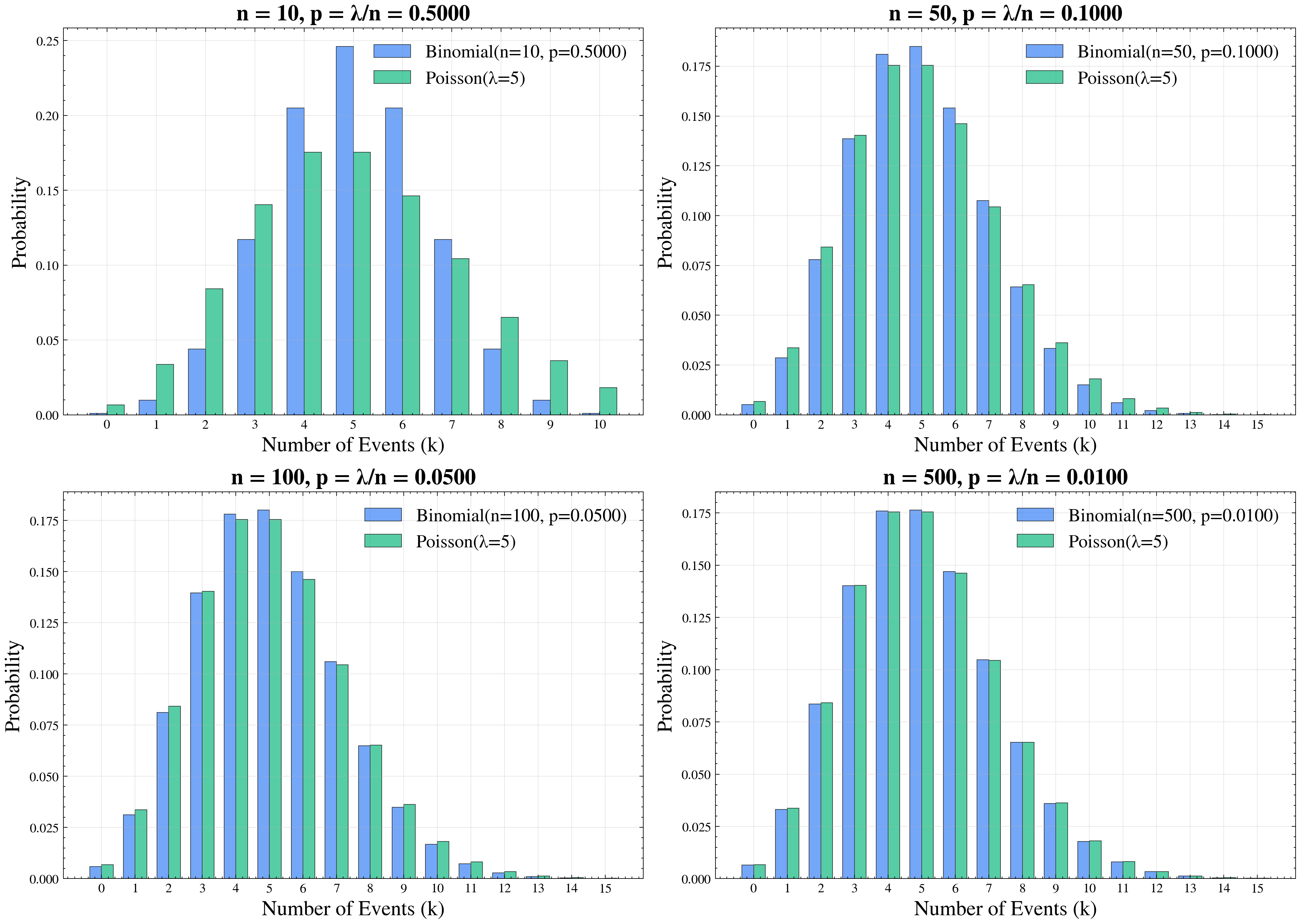
We can simulate this numerically as well. The figure provides a visual confirmation of the theory: as the number of trials increases and the success probability decreases to keep constant, the Binomial distribution (blue bars) gradually aligns with the Poisson distribution (green bars).
Once we accept this limit, the Poisson process becomes much more intuitive. Each of its key properties emerges naturally from the Bernoulli process:
Counts in disjoint intervals are independent: In the Bernoulli world, events in separate time slices are independent by construction. As we shrink the time intervals, this independence persists, meaning that the number of events in non-overlapping periods remains independent in the limit.
The expected number of events grows linearly with time: Each tiny interval contributes a small probability of an event. Summing over intervals gives an expected total of events per time window. If we double the length of the time window, we double the number of intervals and therefore double the expected count. This linearity arises directly from how we scaled the Bernoulli trials.
Waiting times between events become exponential: In discrete time, the number of intervals until the next success follows a geometric distribution. As the interval size shrinks and , the geometric distribution converges to the exponential distribution, giving the Poisson process its memoryless interarrival times.
None of these properties are assumptions added on top of the model. They are inherited automatically from the simple, independent Bernoulli trials we started with. This makes the Poisson process not just mathematically convenient, but a natural description of random arrivals when we zoom in on time and treat events as rare and independent. In this sense, the Poisson model is not imposed on reality, but naturally emerges from it.